Data Structures Fundamentals
Data Structures Explained here:
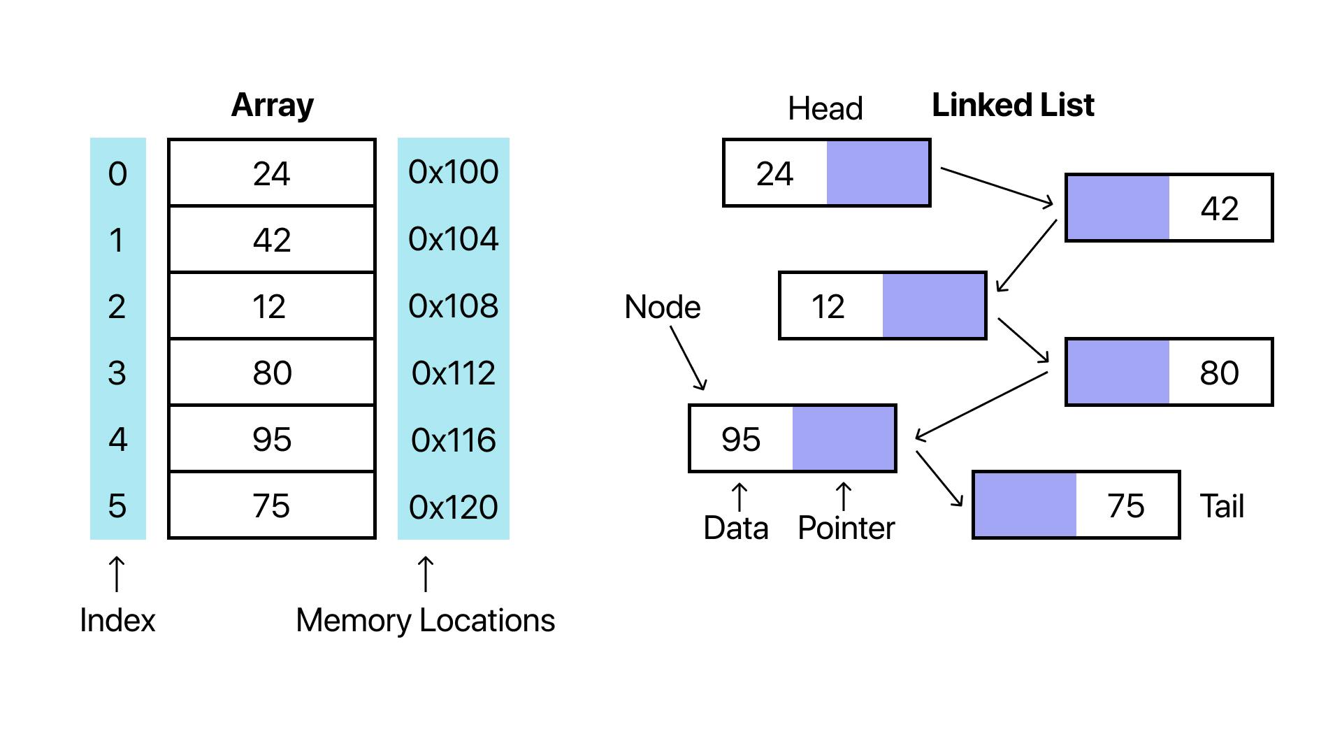
Arrays
Ordered collections of data, typically the data is of similar type but some languages allows for different data types.
Similar type example using C programming language:
#include <stdio.h>

int main() {
  int arr = [1, 2, 3, 4, 5]
  return 0;
}
Different type example using Python programming language:
arr = ["Daniel", True, "James", 10]In some programming languages like Python, Arrays are also referred to as Lists
Array Advantage
It’s very easy to find any element in an array as each element in array is assigned a number called index which is zero-based. The time complexity of finding array element is O(1).
Zero-based indexing starts at 0 (zero).
Array Disadvantage
Longer time needed for inserting or deleting elements (O(n))
Array Memory
Arrays are stored in contigous memory (each element of array are next one to another in memory). If a new element is added in the middle of the array, the entire array must shift down.
But what if there was already something in the next memory address? The array’s memory will have to be reallocated to an entirely new space where all of the elements fit.
Arrays indeed are not very efficient data structure for insertion or deletion but very efficient for item finding.
Linked Lists
Arrays vs Linked Lists
Arrays are fast at reading, but slow at inserting or deleting. On the other hand, Linked Lists are slow at reading but fast at inserting or deleting.
Complexity for reading of a Linked List is O(n) while for inserting or deleting is O(1) which is the exact opposite for an Array.
Linked Lists are similar to Arrays that they store ordered lists of data elements. However, a huge difference is in the way they are stored in the memory.
Memory of Linked Lists
Each element of a Linked List has a pointer. Therefore, elements of Linked List don’t have to be stored beside each other. We can store the next element in any location.
Pointer is basically the address of the next element.
Linked Lists Advantage
Because Linked Lists use pointers, it’s really fast to do insertion and deletion with complexity of O(1).
To add new element:
- Find free spot in memory
- Have the previous element point to it
To delete an element:
- Delete the element
- Have the previous element point to the one ahead of the element just deleted
Linked Lists Disadvantage
Elements don’t have indexes. This means, to find an element, we have to go through the list starting from the beginning with complexity of O(n).
Steps to read an element in Linked List:
- Find the first element
- See where it points
- Go to the second
- See where it points
- Repeat to the next one until the element is found
Hashmaps
Hashmaps are essentially the same as Arrays, except we can choose what the “index” is. The key and its value are commonly known as Key-Value pairs. Hashmaps are sometimes called Hash tables or Dictionaries in Python.
Index in Hashmaps is called Key.
Hashmaps Advantages
Hashmaps are unordered. Hashmaps are fast for both inserting and deleting O(1). However, the real advantage of using Hashmaps are the ability to search quickly O(1).
For Arrays, we’ll have to know the index for each one to read it. But, for Hashmaps, if we make the keys countries for example we can just look up the country to find the capital city associated with it. Example:
{
  "Japan": "Tokyo",
  "London": "England",
  "United States": "Washington D.C."
}
Stacks
 (Image: Stack and Queue)
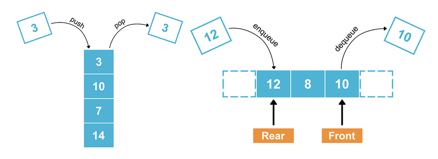
The simplest way to understand a stack is like a stack of plates. Stacks are called LIFO structures.
LIFO or Last In First Out means the last element goes on top of the stack. When you grab something from the stack, the first one taken is the last one added (the top of the stack).
Three operations of stack:
- Push - O(1), adds new element to the stack
- Pop - O(1), removes the top most element of the stack
- Peek - O(1), taking a look of what the top-most element from the stack is.
Queues
Queues are the opposite of a stack. The simplest way to think of a queue is a line at grocery store. Queues are FIFO structure.
FIFO or First In First Out means the first item in the line will get served first, and every item that joins the queue goes at the end.
Three operations of queues (very similar to stacks’):
- Enqueue - O(1), adding new element at the back of the queue
- Dequeue - O(1), element at the front of the queue is removed
- Front - O(1), take a look at the front-most element at the queue
Queues are more oftenly used than stacks, especially in real world programming.
Trees
Trees have nodes, which are connected to each other by edges. The first node in a tree is called root node.
Nodes have parent-child direction where one node is a parent node which leads to another node (child node). People refer to parent nodes just as regular node while child node as leafs.
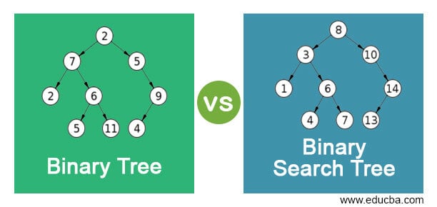
Binary Tree is a tree where each parent node has up to two children nodes. Binary Search Tree is a type of Binary Tree where all left children nodes are less than the parent node and right children nodes are greater than the parent node.
Binary search trees enable easy search through large amounts of ordered values O(log n).
Graphs
Basically models for a set of connections. Like trees, graphs are made up of nodes and edges. In fact, trees and linked-list are technically types of graphs.
Graphs have far less restrictions than trees. No neighbour limit (Nodes can be connected to any amount of neighbours). Graphs can be directed where nodes point to other nodes but could also be undirected.
Some graphs have cycles where two nodes both point to each other. The edges between nodes can also be weighted, where the path has a value associated with it.
Graphs are very complicated. People often call it one of the hardest data structures to learn.